Introduction to Recursion

A Basic Example

Recursion is a strategy that can be applied to problems that have recursive structure. A problem has recursive structure if the problem to be solved can be expressed in terms of a smaller version of the problem.

One of the examples that the author shows in chapter five is the function pow(x,n), which computes xⁿ. This function has a fairly obvious interative implementation

double pow(double x,unsigned int n) {
  double product = 1.0;
  for(unsigned int k = 0;k < n;k++)
    product = product*x;
  return product;
}

This problem also has recursive structure, because the problem (computing xⁿ) can be expressed in terms of a smaller version of the same problem via the relation

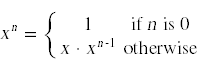
This simple, recursive relationship leads immediately to a recursive implementation of this function in C++:

double pow(double x,unsigned int n) {
  if(n == 0)
    return 1.0;
  return x*pow(x,n-1);
}

This captures the spirit of the recursive mathematical relationship. What we see in this code is an example of a recursive function call: a situation where a function is calling itself with a slightly different parameter.

This is perfectly legitimate programming practice, but you do have to watch out for one very important problem, infinite recursion. An important ingredient in both the recursive definition and the function is the presence of a base case test that stops the recursion when the problem has become simple enough to solve without further recursion.

The initial recursive solution does not offer much of an advantage over the iterative solution. In particular, because of the additional overhead involved in making function calls, the performance of the recursive solution is actually worse than the iterative solution. The great advantage in the recursive solution is that it opens up the possibility of more efficient recursive solutions. Here is another way to define the power operation

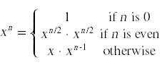
This leads to a recursive function that is vastly more efficient than either of the two previous solutions.

double pow(double x,unsigned int n) {
  if(n == 0)
    return 1.0;
  if(n % 2 == 0) {
    double y = pow(x,n/2);
    return y*y;
  }
  return x*pow(x,n-1);
}

For example, if n is 175, this version of the solution will require 13 multiplications instead of the 175 multiplications required by either of the previous solutions.

Divide and Conquer Recursion

Many problems involving lists have a natural recursive structure. We call problems that can be solved by breaking a list into into smaller pieces and solving recursively divide and conquer problems.

Binary search

Binary search is the classic divide and conquer problem. This function assumes that the vector A contains a list of items sorted in ascending order. A simple strategy to search such a list efficiently is to go to the middle of the list. If the item in the middle of the list is less than the item we are searching for, we can continue the search recursively in the left half of the list. By immediately eliminating half the list, we can dramatically reduce the amount of work we have to do. Coupling this idea with recursion leads to a very efficient solution.

bool search(const vector<string>& A,const string& word) {
  return search(A,word,0,A.size() - 1);
}

bool search(const vector<string>& A,const string& word,
            int start,int end) {
  if(end <= start) // base case
    return (A[start] == word);
  else {
    int mid = (start + end)/2;
    if(A[mid] < word)
      return search(A,word,mid + 1,end);
    else if(A[mid] > word)
      return search(A,word,start,mid - 1);
    else
      return true;
    }
}

This example also demonstrates another feature that is common in recursive solutions. The solution consists of two functions: a recursive function that requires a number of parameters to do its work correctly, and a second, simpler function that starts the recursion. The second function is commonly called a wrapper function.

Quicksort

Perhaps the most famous recursive algorithm designed to operate on lists is quicksort. The quicksort algorithm was developed in 1965 by C.A.R. Hoare, and is probably the most effective general-purpose sorting algorithm for arrays. Here is the source code for one implementation of quicksort.

void swap(int &a, int &b)
{
  int temp = a;
  a = b;
  b = temp;
}

int median(vector<int> & a,int first,int last)
{
    int mid=(first+last)/2;

    if (a[first] < a[mid])
    {
      if (a[mid] < a[last])
        return mid;
      else if (a[first] < a[last])
        return last;
      else
        return first;
    }
    else
    {
      if(a[first] < a[last])
        return first;
      else if(a[last] < a[mid])
        return mid;
      else
        return last;
    }
}

int partition(vector<int> & a,int first,int last)
{
    int p=first;
    
    swap(a[first],a[median(a,first,last-1)]);  
    int piv = a[first];
    
    for(int k=first+1;k<last;k++)
    {
      if (a[k] <= piv)
      {
        p++;            
        swap(a[k],a[p]);
      }
    }
    swap(a[p],a[first]);
    return p;
}

void quickSort(vector<int> & a,int first,int last)
{
  if (last - first > 20)
  {
    int piv = partition(a,first,last);
    quickSort(a,first,piv);
    quickSort(a,piv+1,last);
  }
  else
  {
    selectionSort(a,first,last);
  }
}

void quickSort(vector<int>& a)
{
  quickSort(a,0,a.size());
}

Quicksort consists of several parts. The quickSort function above with three parameters is the main recursive function that is responsible for running the algorithm. A key step in the quicksort process is the partition step, which is implemented by the partition function above. The partition step takes a range of the array and rearranges it to make it closer to being sorted. To partition, we start by selecting one of the values in the range and making it be the pivot value. We then rearrange the values in the range into numbers that are less than or equal to the pivot, the pivot, and numbers greater than the pivot. The numbers that end up in the sub-ranges on either side of the pivot are not sorted, but the entire range does end up being slightly closer to being perfectly sorted after each partition.

The partition step then combines with recursion to finish the job. After partitioning the range, we recursively sort the two sub-ranges created by the partition step. This divide and conquer strategy is effective at sorting the entire array.

The recursion works most efficiently in cases in which the two sub-ranges generated have roughly equal sizes. To give a better chance of producing this result, it helps to pick a good pivot value. This implementation uses a median of three strategy to improve the odds of picking a good pivot. We examine the elements at the beginning, the middle, and the end of the given range, and select the median of those three numbers to be the pivot value. That improves the odds of success above the simple approach of always arbitrarily using the first, middle, or last value in the range as the pivot.

The final detail is setting up an appropriate base case. One obvious base case would be to stop when the range [first,last) has size 1 or smaller. The implementation of quicksort shown here simply stops dividing the array into sub-ranges when the range it is handed has size smaller than 20. For ranges that small, any simple sorting algorithm will suffice, so the base case is to call selectionSort to handle any small sub-ranges created by the divide-and-conquer process.