Reinforcement Learning
In reinforcement learning (RL) an agent learns to operate in an environment to obtain rewards. The goal of the agent is to improve its performance over time and obtain higher rewards.
How RL differs from Supervised Learning
The main paradigm we have used to train neural networks this term is supervised learning (SL). In this paradigm we train a network to perform a task by showing it many examples of what it looks like to solve the task, and the network learns the task by using gradient descent to minimize a loss term.
In reinforcement learning (RL) we are still be going to do some of the same things. We will still be constructing examples and training networks on those examples, but there will be one major difference. In RL the training data will not exist ahead of time. Instead the agent we will be training will generate its own training data, and we will be curating the training data to reinforce successful behaviors while suppressing unsuccessful behaviors.
A simulated environment
In the examples we will be working with in this lecture we will be using the gymnasium python package to supply the environments our agents will work in. The gymnasium package allows us to set up simulation environments in which agents will participate in a series of rounds. At each round the simulation will track a system state, and update that state in reponse to the agent's actions. At each round the environment will give the agent an observation of the system state and then ask the agent to choose an action for the current round. Once the agent has chosen an action to perform the environment will respond by computing a new system state and possibly giving the agent a reward for their most recent action.
The main challenge that agents face in RL scenarios is that rewards may be far removed in time from any individual action choice. For example, if we are training an agent to play chess, the only reward available may be a reward of 1 point when the agent wins the game. In this first lecture we will work with two examples in which the reward is less far removed from agent actions. In the first example below the agent will get a single point for each round that they manage to stay alive, while in the second example we will train an agent to play the Atari Breakout game: in that game a player has to move a paddle to hit a ball into a wall to knock out bricks. The agent will get an immediate reward of one point for each brick they knock out.
The Cartpole example
In the Cartpole game we train an agent to keep a pole upright on a cart that can move right and left.
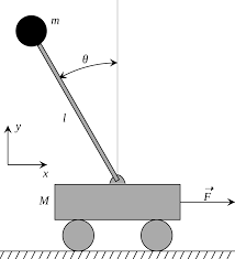
The pole is attached to the cart via a hinge at the base of the pole. At each round of the game the agent can choose to push the cart to the right or the left. To help the agent make decisions about what to do, the environment will provide state information in the form of information on the velocity of the cart, the angle that the pole makes from the vertical, and the angular velocity for the pole. The agent's goal is to keep the pole upright for as many rounds as possible.
A random strategy
For our first solution we are going to use a purely random strategy: at each round of the game the program will randomly push the cart right or left. This strategy is not very effective, and usually only manages to keep the pole from falling over for about 10 time steps.
The example cartpole code below is adapted from the book Deep Reinforcement Learning Hands-On, 3rd Edition by Maxim Lapin.
import gymnasium as gym

if __name__ == "__main__":
    env = gym.make("CartPole-v1")

    total_reward = 0.0
    total_steps = 0
    obs = env.reset()

    while True:
        action = env.action_space.sample()
        observation, reward, terminated, truncated, info = env.step(action)
        total_reward += reward
        total_steps += 1
        if terminated or truncated:
            break

    print("Episode done in %d steps, total reward %.2f" % (
        total_steps, total_reward))
The code starts by setting up an environment to play the game. To start the game we call the environment's reset() method, which returns an observation about the state of the game at start. Each environment contains an action_space member variable which contains information about the actions that are available to the player. The action space object offers a sample() method we can call to select an action at random.
To take a single step in the environment we call the environment's step() method, passing it the action we want to take. The environment will respond with a tuple that contains the next observation, the reward for this step, and other information. The cartpole environment will give us a reward of 1 for each step that the pole remains upright.
Training a network to play the game
In the second version of this problem we will instead use a neural network to decide what action to take at each step.
Specifically,
- The network will take observations as its inputs and output a probability distribution over all possible actions.
- On each round we will feed the current observation to the network and have it output a probability distribution.
- We then sample from that distribution to get our next action.
We note several key points here:
- At start the network will have random weights and will be spitting out probability distributions at random. This causes the system to use more or less random actions at start.
- Next, we will be watching the results produced by the network. Whenever we see the network produce a sequence of moves that results in the pole staying upright for a longer than average span of moves, we make a record of all of the moves in that sequence and train the network on that record. At the same time, we will eventually remove less successful runs from the record and stop training on them.
- Over time the network will learn to produce outputs that result in better and better runs.
- Even when the network gets trained we will still be introducing a small amount of randomness by sampling from the output distribution. This will allow our system to continue exploring the state space somewhat even after the network converges to a strategy.
Here now is the code to implement this more advanced strategy:
import gymnasium as gym
from collections import namedtuple
import numpy as np

import torch
import torch.nn as nn
import torch.optim as optim


HIDDEN_SIZE = 128
BATCH_SIZE = 16
PERCENTILE = 70


class Net(nn.Module):
    def __init__(self, obs_size, hidden_size, n_actions):
        super(Net, self).__init__()
        self.net = nn.Sequential(
            nn.Linear(obs_size, hidden_size),
            nn.ReLU(),
            nn.Linear(hidden_size, n_actions)
        )

    def forward(self, x):
        return self.net(x)


Episode = namedtuple('Episode', field_names=['reward', 'steps'])
EpisodeStep = namedtuple('EpisodeStep', field_names=['observation', 'action'])


def iterate_batches(env, net, batch_size):
    batch = []
    episode_reward = 0.0
    episode_steps = []
    obs = env.reset()[0]
    sm = nn.Softmax(dim=0)
    while True:
        obs_v = torch.FloatTensor(obs)
        act_probs_v = sm(net(obs_v))
        act_probs = act_probs_v.data.numpy()
        action = np.random.choice(len(act_probs), p=act_probs)
        next_obs, reward, terminated, truncated, info = env.step(action)
        episode_reward += reward
        step = EpisodeStep(observation=obs, action=action)
        episode_steps.append(step)
        if terminated or truncated:
            e = Episode(reward=episode_reward, steps=episode_steps)
            batch.append(e)
            episode_reward = 0.0
            episode_steps = []
            next_obs = env.reset()[0]
            if len(batch) == batch_size:
                yield batch
                batch = []
        obs = next_obs


def filter_batch(batch, percentile):
    rewards = list(map(lambda s: s.reward, batch))
    reward_bound = np.percentile(rewards, percentile)
    reward_mean = float(np.mean(rewards))

    train_obs = []
    train_act = []
    for reward, steps in batch:
        if reward < reward_bound:
            continue
        train_obs.extend(map(lambda step: step.observation, steps))
        train_act.extend(map(lambda step: step.action, steps))

    train_obs_v = torch.FloatTensor(train_obs)
    train_act_v = torch.LongTensor(train_act)
    return train_obs_v, train_act_v, reward_bound, reward_mean


if __name__ == "__main__":
    env = gym.make("CartPole-v1")
    obs_size = env.observation_space.shape[0]
    n_actions = env.action_space.n
    net = Net(obs_size, HIDDEN_SIZE, n_actions)
    objective = nn.CrossEntropyLoss()
    optimizer = optim.Adam(params=net.parameters(), lr=0.01)

    for iter_no, batch in enumerate(iterate_batches(
            env, net, BATCH_SIZE)):
        obs_v, acts_v, reward_b, reward_m = \
            filter_batch(batch, PERCENTILE)
        optimizer.zero_grad()
        action_scores_v = net(obs_v)
        loss_v = objective(action_scores_v, acts_v)
        loss_v.backward()
        optimizer.step()
        print("%d: loss=%.3f, reward_mean=%.1f, rw_bound=%.1f" % (
            iter_no, loss_v.item(), reward_m, reward_b))
        if reward_m > 199:
            print("Solved!")
            break
Here are some observations about this code:
- The
iterate_batches()function runs game episodes until it has collected enough data to form a batch of game episodes. iterate_batches()is an example of a Python generator function. In place ofreturnit usesyield. When you hit ayieldstatement you will return a result. The next time the generator function gets called it will pick back up where theyieldstatement left off.- The batches spit out by
iterate_batches()contain both successful runs and unsuccessful runs. Thefilter_batch()function retains only the data from longer runs and returns a tuple containing all of the steps it collected from those successful runs.
Learning to play Atari games
In 2015 several researchers from DeepMind published a paper in Nature in which they described building a reinforcement learning system with a neural network that could spontaneously learn to play Atari video games expertly. In these notes I will explain how they did this, and show some example code to implement their system in PyTorch.
Here is a link to a YouTube video showing the system learning to play Breakout.
The Q table
The goal in games is to achieve a high score. In the world of reinforcement learning, points scored in a game are considered to be rewards granted by the game environment. The goal of an intelligent agent is to develop a strategy to maximize their rewards.
In reinforcement learning, the Q table is a table that records the expected future reward Q(s,a) for each combination of a state s and an action a that the agent can take from that state. In cases where the available states in a system are finite and discrete, these values truly can be stored in a table whose rows are the possible states s of the system and whose columns are the possible actions a that an agent can perform.
The entries in the Q table satisfy the Bellman equality:
Q(s,a) = r(s,a) + γ V(s')
where r(s,a) is the immediate reward for executing action a from state s, s is the state that results from performing action a from state s, and V(s
 ) is the maximum future reward from state s':
V(s') = maxa Q(s',a)
Another factor in these equations is the γ factor, which is used to discount the future. Each time we take a step back in time from a place where we can receive a reward of r, we discount that future reward by the γ factor: this biases the system toward wanting to gain rewards sooner rather than later.
These are the equations that the entries of the Q table have to satisfy, but they unfortunately do not tell us how to actually compute the values of the table. For this, we typically use an iterative update strategy to fill out the table. In this strategy we do the following:
- We start out by putting a 0 in all cells in the table.
- We operate in the environment, carrying out actions a from states s that we encounter.
- Occasionally, we will carry out an action that leads to an immediate reward. As soon as we get that reward r(s,a) we go to entry Q(s,a) in the table and update it with the immediate reward r(s,a) that we just got.
- Once rewards start to appear in the table, they can also start to propagate outward. For example, suppose we enter a state sp and discover that there is an action ap that can take us to a state s. If there is an action a such that Q(s,a) = 1, then V(s) will be 1, and then Q(sp,ap) = r(sp,ap) + γ V(s) = 0 + γ
This plan actually has theoretical support, since Bellman showed that if we carry out these updates to the Q table for enough rounds, eventually the values across the whole table will converge to the correct values.
The Q function and the Q network
The problem with the theory I set out in the previous section is that it rests on an assumption that sometimes is not true: we assumed that the system we were working with had a finite set of discrete states. Some of the environments we would like to operate in violate that assumption, either because the environment does not have discrete states or it has so many discrete states that Q table becomes unworkably large. In those cases we can instead fall back on trying to construct a Q function instead of a Q table. A Q function would still satisfy the Bellman equality.
If we decide to replace the Q table with a Q function it is only a small jump from there to imagine building a Q neural network that would have the task of computing that function. (This sort of network is usually referred to as a deep-Q network.) We can even train that network to learn the Q function by using an update scheme very similar to the one I set out above:
- We start with an initial random set of weights in the network.
- We operate in the environment, carrying out actions a from states s that we encounter. Each time we carry out an action we construct an input/target pair consisting of (s,a) and the immediate reward r(s,a) that we just got combined with γ maxa Q(s
 ,a), where we use the network to compute Q(s
 ,a).
- We train the network on all of the input/target pairs we collected.
The next thing we need to think about is choosing actions: until we have a strategy to do this we can't operate in the environment. Fortunately, this where the Q network can help us. When we arrive at a state s and we have select a next action a we can use our Q network to compute Q(s,a) for every possible a, and then select the action that produces the largest possible Q value.
Another strategy that we use to supplement this plan is the ε-greedy strategy. In this strategy we set up a parameter ε that starts out close to 1. On each round we pick a real number at random from the interval (0,1): if that number is larger than ε we use the Q network to pick our next action, otherwise we select our next action at random. After each round we decrease ε slightly, so that over time the Q network determines our actions more often as it learns the correct Q values. This gives the system the opportunity to explore the state space early on and eventually lean more and more heavily on the network to control our actions.
Learning to play Atari games
The main example we are going to look at today is the example of using a deep-Q network to train an agent to play the Atari breakout game.
Here is an article that shows a pytorch implementation of a deep-Q network that can learn to play the Pong game. This solution could easily be rewritten to play breakout instead.
The state information that the system learns from is composed of images of the video game screen. Specifically, the state space consists of stacks for four frames at a time. We have to include multiple frames in the state information because a single image frame would only show where the ball and the paddle are located. We need multiple frames so the system can determine where the ball is moving.
The code runs a series of episodes, where each episode is a complete game of breakout. In each episode we use a combination of ε-greedy random moves and moves determined by using the network to give us an estimate for Q(s,a) for each possible action and then selecting the action with the largest Q value. As we play the game, we store a record of states, actions selected, and rewards obtained. (This record is known as a replay buffer.)
To train the Q network we make random samples from the replay buffer and compute targets q = r(s,a) + γ V(s') for each sample (we use the Q network to estimate V(s') for this step). We then train the Q network with inputs (s,a) and targets q.
Another feature of the example that is significant is the use of two networks. The second network, which we call the target network, is only used to compute the V(s) estimates when needed. The first network does everything else, and also gets trained on new examples from the replay buffer periodically. Finally, after every 10000 frames of game play we copy the weights from the Q network we have been training to the target network. The reason for this unusual two network strategy is to improve the stability of our Q learning: since Q(s,a) and V(s) related recursively, sometimes updates to Q(s,a) can cause an unwelcome feedback loop between these two factors. The solution to this problem is to break the feedback loop by only updating the Q(s,a) network and temporarily keeping the network we use to compute V(s) frozen. Eventually updates to Q(s,a) will transfer to V(s) when we copy the weights from the Q network to the target network.