Proving that algorithms are correct
In the lecture for chapters 21 and 22 I gave some reasons for why you should believe that the algorithms there are correct. Those reasons were helpful in understanding how the algorithms worked, but did not constitute a formal proof that the algorithms were correct. In these notes I am going to introduce you to a proof framework that can be used to prove that iterative algorithms are correct. Once we have seen a couple of basic examples of how the frame is used in practice we will revisit the algorithms from chapters 21 and 22 and give formal proofs of correctness for those algorithms.
Proving that a loop is correct
Almost all iterative algorithms do most of their interesting steps in one or more loops. In these notes I am going to introduce you to a proof framework that can be used to prove that a loop does what we claim it does.
To help standardize our proof framework, all of the loops we will be working with will have the following generic form:
<initialization>
while(!<termination>) {
  <body>
}
Here is what the various parts of the loop will do:
- The
<initialization>code will set up any variables needed by the loop. Most loops are driven by a loop variable, so at a minimum we will need to give the loop variable an initial value. - The loop is controlled by a
<termination>condition, which is a boolean expression. The loop runs until the<termination>condition is true. - The loop also has a
<body>.
Not every loop that we look at will use a while loop, but every loop can be re-written as a while loop.
The next thing we will do is to introduce a number of additional boolean expressions, called predicates. The purpose of these predicates is to help express what we think is true at various points in the loop code.
Specifically, we will be working with three main predicates:
- An initialization predicate that says what is true right after
<initialization>and before the loop starts. - A goal predicate that says what is true at the end of the loop.
- A loop invariant that says what is true before we run the
<body>. The loop invariant should still be true after the<body>runs.
With these three predicates in place each proof will consist of these steps:
- Show that the initialization predicate is true right after <initialization>.
- Show that the initialization predicate implies the loop invariant.
- Show that if the loop invariant is true and the termination condition is true then the goal predicate has to be true.
- Show that the loop invariant is still true after each pass through the body. That is, if the loop invariant is true before we run the <body> then it will still be true after the <body> runs.
Example: Quicksort partition
Here once again is the pseudocode for Quicksort:
QUICKSORT(A,p,r)
  if p < r
    q = PARTITION(A,p,r)
    QUICKSORT(A,p,q-1)
    QUICKSORT(A,q+1,r)

PARTITION(A,p,r)
  x = A[r]
  i = p-1
  for j = p to r-1
    if A[j] <= x
      i = i + 1
      exchange A[i] with A[j]
  exchange A[i+1] with A[r]
  return i + 1
Quicksort has two parts, a recursive function QUICKSORT(A,p,r) and an iterative functionPARTITION(A,p,r). For my first example I am going to prove that the loop in the partition function does what we expect.
The first step is to rewrite the code slightly to use a while loop instead of a for loop.
PARTITION(A,p,r)
  x = A[r]
  i = p-1
  j = p
  while (j < r)
    if A[j] <= x
      i = i + 1
      exchange A[i] with A[j]
    j = j + 1
  exchange A[i+1] with A[r]
  return i + 1
Predicates
Next, we construct an appropriate goal predicate:
<goal> = (A[p..i] <= x) and (A[i+1..r-1] > x)
If this is true, we can then safely make A[i+1] trade places with A[r] and end up with the overall goal of the partition function:
<partition goal> = (A[p..i] <= x) and (A[i+1] = x) and (A[i+2..r] > x)
The termination condition for the loop is essentially
<termination> = (j = r)
Another predicate that is easy to write down is the initialization predicate:
<initialization> = (i = p-1) and (j = p)
Finally, we are going to need a loop invariant. This is the least obvious part of the process, and requires some experience to get right. For this example I will simply say what the loop invariant is, and then we will go on to show that it works in the proof. Very often loop invariants are a somewhat weakened version of the goal predicate. Here is the loop invariant I will use:
<invariant> = (A[p..i] <= x) and (A[i+1..j-1] > x)
Proof of correctness
Now we are in a position to construct the proof. Here are the relevant steps:
1) <initialization> implies <invariant>: to show this it suffices to plug i = p-1 and j = p into the invariant:
(A[p..p-1] <= x) and (A[p..p-1] > x)
This results in a predicate that is trivially true, since both of the ranges mentioned here are empty.
2) <invariant> and <termination> implies <goal> is also easy:
(A[p..i] <= x) and (A[i+1..j-1] > x) and (j=r) => (A[p..i] <= x) and (A[i+1..r-1] > x)
3) <invariant> is still true after <body>. Before we run any of the <body> code we can count on the invariant being true.
(A[p..i] <= x) and (A[i+1..j-1] > x)
The complication is that the <body> code may potentially change the values of i and j. The invariant may be true for the old values of i and j, but it may no longer be true after updating these variables.
Let's start by focusing on one thing that always happens in the body:
j = j + 1
The danger here is that if A[j] <= x, then incrementing j would cause (A[i+1..j-1] > x) to no longer be true.
The fix for this problem is to add logic to the body that anticipates this and fixes the problem. That is the motivation behind this chunk of the logic:
if A[j] <= x
  i = i + 1
  exchange A[i] with A[j]
The fix here is to watch out for the bad case and then fix it by making A[i+1] and A[j] trade places. This is safe to do, because A[i+1] > x and A[j] <= x.
After the fix (which also involves incrementing i) we come back to the invariant being true.
Nested loops example
Now that we have seen a basic example, it is time to turn our attention to a problem that features another common phenomenon in iterative algorithms, a nested set of loops. In this next example we are going to look at a sorting algorithm called bubble sort. This is an example of a relatively inefficient sorting algorithm, but it has enough complexity to make it worth our time to study it.
In the discussion below, the notation A[1..i] ≤ A[i+1..n] stands for "every element in the range A[1..i] is less than or equal to every element in the range A[i+1..n]." Further, if one or both of the two ranges is empty, the statement is understood to be trivially true.
The Code
Suppose A[1..n] is an initially unsorted array of integers. Here is some code to sort the array using the bubble sort algorithm.
i = 1;
while(i <= n)
  {
  j = n;
  while(j > i)
    {
    if(A[j] < A[j-1])
      {
      temp = A[j-1];
      A[j-1] = A[j]
      A[j] = temp;
      }
    j--;
    }
  i++;
  }
Analysis of the inner loop
Since this code is structured as a pair of nested loops, we will apply the proof technique to both loops in turn. Since the outer loop will rely on the inner loop, we start our analysis with the inner loop.
<goal> = "A[i] ≤ A[i+1..n]"
<invariant> = "A[j] ≤ A[j+1..n]"
<initialization> = "j = n"
<termination> = "j = i"
The invariant is trivially true at initialization time because the range A[j+1..n] is empty. It is also easy to see that <invariant> + <termination> = <goal>. The only thing to prove is that the loop body maintains the invariant.
At the beginning of the loop body we have that A[j] is the smallest element in A[j..n]. If A[j] is also smaller than A[j-1], we make the two trade places so that now A[j-1] ≤ A[j..n]. Otherwise, we leave A[j-1] in place so that once again A[j-1] ≤ A[j..n]. After doing the decrement of j at the end of the loop body the inequality looks like the invariant again because the decrement effectively replaces j-1 with j.
Analysis of the outer loop
<goal> = "A[1..n] is sorted"
<invariant> = "(A[1..i-1] is sorted) and (A[1..i-1] ≤ A[i..n])"
<initialization> = "i = 1"
<termination> = "i = n + 1"
The invariant is trivially true at initialization time because the range A[1..i-1] is empty. <invariant> + <termination> = <goal> because at termination time A[1..i-1] = A[1..n] and the range A[i..n] is empty at termination. That means that at termination the invariant reduces to "(A[1..n] is sorted) and (true)", which is the same as <goal>.
At the beginning of the outer loop body we have "(A[1..i-1] is sorted) and (A[1..i-1] ≤ A[i..n])". After execution of the inner loop we also have "A[i] ≤ A[i+1..n]". The condition (A[1..i-1] ≤ A[i..n]) implies that A[i-1] ≤ A[i], because A[i] is just one element of the larger range A[i..n] and A[i-1] is a representative of the range A[1..i-1]. Combining (A[1..i-1] is sorted) with (A[i-1] ≤ A[i]) gives (A[1..i] is sorted). This maintains the first half of the invariant. Coupling the inner loop goal "A[i] ≤ A[i+1..n]" with (A[1..i-1] ≤ A[i..n]) leads to (A[1..i] ≤ A[i+1..n]), maintaining the second half of the invariant.
After execution of the inner loop we have "(A[1..i] is sorted) and (A[1..i] ≤ A[i+1..n])". Incrementing i at the end of the outer loop body restores the invariant back to the original "(A[1..i-1] is sorted) and (A[1..i-1] ≤ A[i..n])".
Proof of correctness for chapter 21 algorithms
Somewhat surprisingly, the two algorithms that we studied in chapter 21, Kruskal's algorithm and Prim's algorithm, both have the same proof of correctness.
The proof consists of first rewriting both algorithms as an equivalent generic MST Algorithm:
Generic MST
GENERIC-MST(G,w)
  A = ∅
  while A does not form a spanning tree
    find an edge (u,v) that is safe for A
    A = A ⋃ {(u,v)}
  return A
This algorithm leans on some special definitions
- A cut is some subdivision of a collection of vertices into one set S and its complement, V-S.
- An edge crosses the cut if it connects a vertex in S to a vertex in V-S.
- A cut respects a set A if none of the edges in A cross the cut.
- If A is a subset of a MST T and E is an edge, we say that E is safe for A if A ∪ {E} is a subset of an MST T
 .
.
First off, why are both Kruskal and Prim examples of this more generic algorithm? The answer lies in the unique way that each algorithm constructs the sets S on each round. In Prim's algorithm A is just the set of edges we have chosen so far, and the set S is always just the set of vertices we have manage to connect by using the edges in A. For Kruskal we focus on the next edge that Kruskal wants to use. If that edge does not cause a cycle with the edges we have chosen already it will connect to components of the graph together. The trick then is to set S equal to one of those two components and note that the edge we are about to pick is the cheapest edge crossing the cut around S.
The proof of correctness for the while loop in the generic MST algorithm hinges on this theorem:
Theorem 21.1
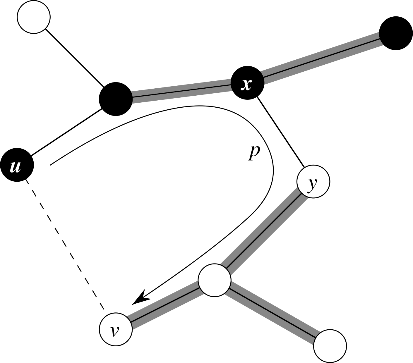
Let G = (V,E) be a connected, undirected graph with a real-valued weight function w defined on E. Let A be a subset of E that is included in some minimum spanning tree for G, let (S,V-S) be any cut of G that respects A, and let (u,v) be a light edge crossing (S,V-S). Then, edge (u,v) is safe for A.
I am going to refer you to the text to read the proof of this theorem, which makes an argument illustrated below.
Proof of correctness for Dijkstra's algorithm
Here again is the pseudocode for Dijkstra's algorithm.
DIJKSTRA(G,w,s)
  INITIALIZE-SINGLE-SOURCE(G,s)
  S = ∅
  Q = G.V
  while Q != ∅
    u = EXTRACT-MIN(Q)
    S = S ⋃ {u}
    for each vertex v ∈ G.Adj[u]
      RELAX(u,v,w)
The proof of correctness for Dijkstra's algorithm leans on the following loop invariant:
When u enters S (and for all time after that), u.d = δ(s,u).
Once again, I am going to direct you to the text to read the details of the proof, which makes use of a comple of important lemmas:
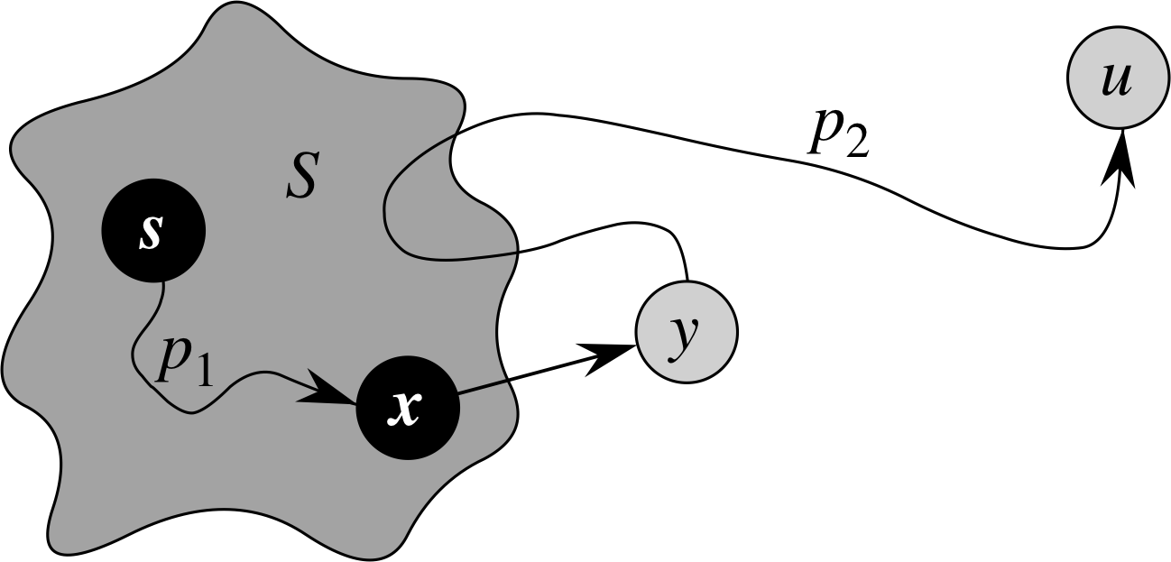
Subpath Lemma (21.1) If s→→u→→v is a shortest path from s to v, then s→→u is a shortest path from s to u.
Convergence Lemma (21.14) If s→→u→v is a shortest path from s to v, and if u.d = δ(s,u) at any time prior to relaxing edge (u,v), then v.d = δ(s,v) at all times afterward.
The proof also leans on a key step that is illustrated by the diagram below.
Proof of correctness for a recursive algorithm
The technique I presented here provides a framework for proving that iterative algorithms are correct. Recursive algorithms are going to require a different approach. Fortunately, there is a method to prove that recursive algorithms are correct that works well across a wide range of examples: we apply proof by induction to the recursion.
To illustrate how this works, let us revisit Quicksort. Here again is the full pseudocode for that algorithm:
QUICKSORT(A,p,r)
  if p < r
    q = PARTITION(A,p,r)
    QUICKSORT(A,p,q-1)
    QUICKSORT(A,q+1,r)

PARTITION(A,p,r)
  x = A[r]
  i = p-1
  for j = p to r-1
    if A[j] <= x
      i = i + 1
      exchange A[i] with A[j]
  exchange A[i+1] with A[r]
  return i + 1
The proof of correctness technique I introduced above allows us to claim that the partition function will do the right thing whenever we call it. To extend this to a proof that the full Quicksort algorithm is correct we construct a proof by induction on the size of the range [p..r] that we are sorting.
Here are the details.
Base case For a range [p..r] with size 0 we will hit the base case in the Quicksort algorithm. That base case does nothing, which is the right thing to do when sorting an array of size 0.
Induction step We assume that Quicksort is able to correctly sort a portion of an array A[p..r] when the size of the range [p..r] < n for some n. We prove that Quicksort can sort a portion of an array A[p..r] when the size of the range [p..r] equals n. Here are some observations:
- Quicksort will start by running the partition algorithm on A[p..r]. This will result in A[p..r] being reorganized into parts A[p,q-1] containing numbers that are less than or equal to A[q], A[p+1..r] containing numbers that are all greater than A[q], and A[q] itself.
- We then apply Quicksort recursively on A[p..q-1] and A[q+1..r]. Since these sub-ranges will both have size < n, the induction assumption allows us to assume that these will be properly sorted.
- Once the subranges are sorted the entire range A[p..r] is correctly sorted.