Consider the problem of finding the area between the graph of the function y = x2 and the x axis between x = 1 and x = 2. The shape bounded by those curves is not a simple geometric shape whose area can be computed easily. The best we can hope for is some sort of estimate of the actual area. Today we are going to study a method used to estimate this area. Eventually this method will even make it possible to compute the area exactly.
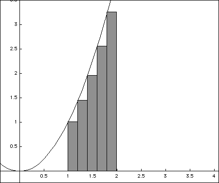
To start the estimation process, imagine subdividing the interval [1,2] into, say, five equal sized subintervals. Over each of the subintervals we draw a rectangle that just touches the graph of y = x2 in one place.
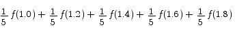
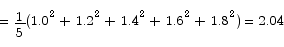
The sum of the areas of the rectangles gives a simple approximation to the area under the curve. Computing the areas of the rectangles is very easy. Each rectangle has a width of (2 - 1)/5 = 1/5 and a height determined by the value of the function  at the left hand endpoint of the sub-interval. The total area is
To make a better approximation, we could use more and skinnier rectangles.
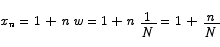
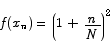
No matter how many rectangles we use, the calculation will always follow the same basic pattern. The typical rectangle starts at some point xn-1 and ends at a point xn. The height of the rectangle is given by  where
where 
The area of the typical rectangle is

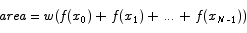
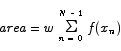
which makes the area of all of the rectangles put together

To make computing this area easier, lets set this up so that all of the rectangles have the same width, w.

In this language, the rectangles in the picture above are generated by picking cn = xn-1.
| (1) |
As we work with these area calculations, we will very often find ourselves working with sums like (1). To save ourselves the work of having to write out these sums in long form, we will introduce a more compact notation, called summation notation, for representing these sums.
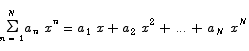
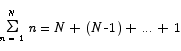
In its most basic form, a summation expression looks like

This expression has several components. The first is the index of summation, n. The index takes a series of different values indicated by the values below and above the  . In this case, the range of values for the index is 1 to N. Following the
  is the summand, an expression which depends on the index of summation. To generate the sum that this expression stands for, we generate every term that results from replacing the index of summation in the summand with on of the values in the range of index values and then add all those terms together.
This is not nearly as complicated as it sounds. A few simple examples will show how the summation notation works.
In summation notation, the quantity we have to compute in (1) can be written
In order to make summations more than a notational convenience, we are now going to introduce a number of basic results concerning calculations with summations.
Since a summation is nothing more than a fancy way to write sums, summations inherit their basic algebraic properties from sums. Here are a couple of those basic properties.
Distributive law The standard distributive law is a rule for multiplying common factors into sums and factoring them out again. In standard form this law is
In summation notation this law looks like
Associative law The associative law basically says that it does not matter what order we perform additions in
In summation notation this law comes up whenever we have a sum of a sum.
In addition to these basic properties, summations also feature some new manipulations.
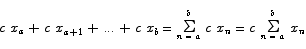
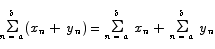
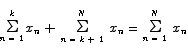
Combining two sums Two sums whose indices of summation and summands match up in just the right way can be combined into a single sum.
Change in index of summation Occasionally we will need to transform a summation by making a change in its index of summation. Here is an example. Consider the sum
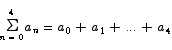
Suppose we did not like the fact that the sum started at n = 0, and instead wanted to transform this into a sum that started with an index value of 1. To accomplish this, we first introduce a new variable, k, that will represent the new index of summation. We want to set things up so that when n = 0 we have instead k = 1, so the obvious relationship we want is
k = n + 1
n = k - 1
With that change of variables, we have to then specify how each part of the summation expression changes.
The resulting summation is

As we work with summations, we will see certain basic problems appear time and again. In this section we will solve three of the most basic summation problems. The result will be three useful standard formulas for working with sums.
The first problem is extremely easy to solve
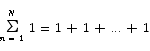
All that we are doing here is to add the same thing to itself a number of times. All that we need to know to compute the sum is how many terms are in the sum. Examination of the starting and ending indices shows that there are N terms in the sum. Thus,

The next problem is a little harder.
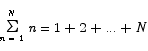
There is a simple trick which will unlock this problem. Since addition is commutative, it does not matter what order we write the terms in the sum. Thus, the sum above is equal to
Notice that when we add the terms in the two sums term by term, we always get the same sum, N + 1. Thus we have that
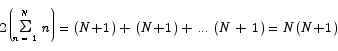
or

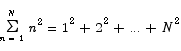
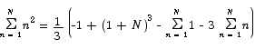
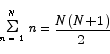
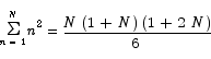
Next I am also going to develop the formula for this sum.
This requires a good deal more cleverness to solve. To solve this problem, we begin by examining a problem which at first glance appears to be harder:
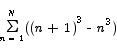
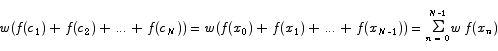
Why consider this problem instead? For starters, it has a special property, called the telescoping sum property, that actually makes it very easy to solve.

If you examine the sum on the right closely, you will see that some serious cancellation is going to happen here. The first part of the first term cancels with the second part of the second term. The first part of the second term cancels with the second part of the third term. In fact, with the exception of the second and the next to the last terms of this sum, everything cancels out.
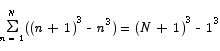
The second thing that is special about this problem is that it has our original problem buried in it. By simple algebra we have
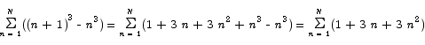
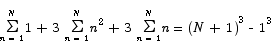
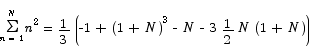
By a series of applications of basic summation properties we can simplify this to
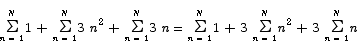
Sitting in this final summation are two expressions whose value we have already computed. The middle term is the thing we want.
Note that it is relatively easy to take the basic idea used in this calculation and compute

for any positive integer k.
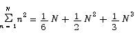
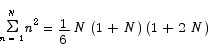
Summary To sum up, the three key formulas we have just developed are

We are now in a position to return to the original area calculation problem and handle it in a slightly more general and more abstract manner. This time around we are going to divide the interval from 1 to 2 into N equal sized sub-intervals. Over each of those subintervals we will place a rectangle whose height was given by the value of the function over the left endpoint. Thus, we have something like
where

and
and hence
Thus the sum we have to compute is
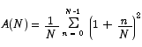
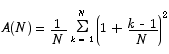
Before we can compute this sum, we have to change the index. All three of the standard formulas we developed above are based on sums whose indices start at 1. Thus we need to make a change of index with
k = n + 1
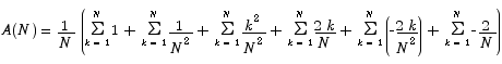
After that change the sum becomes
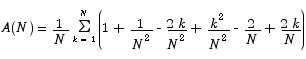
In order to be able to use our formulas from above, we have to do a little algebra first.

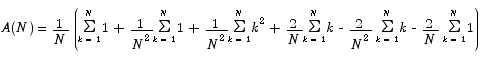
Now we are in a position to apply the summation formulas we developed above.
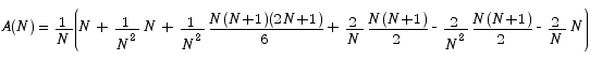
This mess simplifies to
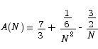
Now that we have an explicit expression that connects the number of subdivisions to the area estimate, we can see how good an estimate we are going to get based on the number of rectangles we use.
| N | A(N) |
|---|---|
| 5 | 2.04 |
| 10 | 2.1850000000000001 |
| 15 | 2.2340740740740741 |
| 20 | 2.25875 |
| 25 | 2.2736000000000001 |
| 30 | 2.2835185185185187 |
We can also see that in the limit of the number of rectangles becoming very large we will get a definite result:
Section 5.1: 4, 5, 22