numpy for Linear Algebra

numpy for matrices and vectors

The numpy ndarray class is used to represent both matrices and vectors. To construct a matrix in numpy we list the rows of the matrix in a list and pass that list to the numpy array constructor.

For example, to construct a numpy array that corresponds to the matrix

we would do

A = np.array([[1,-1,2],[3,2,0]])

Vectors are just arrays with a single column. For example, to construct a vector

we would do

v = np.array([[2],[1],[3]])

A more convenient approach is to transpose the corresponding row vector. For example, to make the vector above we could instead transpose the row vector

The code for this is

v = np.transpose(np.array([[2,1,3]]))

numpy overloads the array index and slicing notations to access parts of a matrix. For example, to print the bottom right entry in the matrix A we would do

print(A[1,2])

To slice out the second column in the A matrix we would do

col = A[:,1:2]

The first slice selects all rows in A, while the second slice selects just the middle entry in each row.

To do a matrix multiplication or a matrix-vector multiplication we use the np.dot() method.

w = np.dot(A,v)

Solving systems of equations with numpy

One of the more common problems in linear algebra is solving a matrix-vector equation. Here is an example. We seek the vector x that solves the equation

A x = b

where

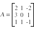
We start by constructing the arrays for A and b.

A = np.array([[2,1,-2],[3,0,1],[1,1,-1]])
b = np.transpose(np.array([[-3,5,-2]])

To solve the system we do

x = np.linalg.solve(A,b)

Application: multiple linear regression

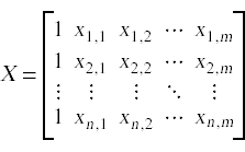
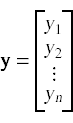
In a multiple regression problem we seek a function that can map input data points to outcome values. Each data point is a feature vector (x₁ , x₂ , …, x_m) composed of two or more data values that capture various features of the input. To represent all of the input data along with the vector of output values we set up a input matrix X and an output vector y:

In a simple least-squares linear regression model we seek a vector β such that the product Xβ most closely approximates the outcome vector y.

Once we have constructed the β vector we can use it to map input data to a predicted outcomes. Given an input vector in the form

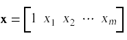
we can compute a predicted outcome value

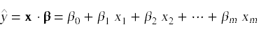
The formula to compute the β vector is

β = (X^T X)^-1 X^T y

In our next example program I will use numpy to construct the appropriate matrices and vectors and solve for the β vector. Once we have solved for β we will use it to make predictions for some test data points that we initially left out of our input data set.

Assuming we have constructed the input matrix X and the outcomes vector y in numpy, the following code will compute the β vector:

Xt = np.transpose(X)
XtX = np.dot(Xt,X)
Xty = np.dot(Xt,y)
beta = np.linalg.solve(XtX,Xty)

The last line uses np.linalg.solve to compute β, since the equation

β = (X^T X)^-1 X^T y

is mathematically equivalent to the system of equations

(X^T X) β = X^T y

The data set I will use for this example is the Windsor house price data set, which contains information about home sales in the Windsor, Ontario area. The input variables cover a range of factors that may potentially have an impact on house prices, such as lot size, number of bedrooms, and the presence of various amenities. A CSV file with the full data set is available here. I downloaded the data set from this site, which offers a large number of data sets covering a large range of topics.

Here now is the source code for the example program.

import csv
import numpy as np

def readData():
    X = []
    y = []
    with open('Housing.csv') as f:
        rdr = csv.reader(f)
        # Skip the header row
        next(rdr)
        # Read X and y
        for line in rdr:
            xline = [1.0]
            for s in line[:-1]:
                xline.append(float(s))
            X.append(xline)
            y.append(float(line[-1]))
    return (X,y)

X0,y0 = readData()
# Convert all but the last 10 rows of the raw data to numpy arrays
d = len(X0)-10
X = np.array(X0[:d])
y = np.transpose(np.array([y0[:d]]))

# Compute beta
Xt = np.transpose(X)
XtX = np.dot(Xt,X)
Xty = np.dot(Xt,y)
beta = np.linalg.solve(XtX,Xty)
print(beta)

# Make predictions for the last 10 rows in the data set
for data,actual in zip(X0[d:],y0[d:]):
    x = np.array([data])
    prediction = np.dot(x,beta)
    print('prediction = '+str(prediction[0,0])+' actual = '+str(actual))

The original data set consists of over 500 entries. To test the accuracy of the predictions made by the linear regression model we use all but the last 10 data entries to build the regression model and compute β. Once we have constructed the β vector we use it to make predictions for the last 10 input values and then compare the predicted home prices against the actual home prices from the data set.

Here are the outputs produced by the program:

[[ -4.14106096e+03]
 [  3.55197583e+00]
 [  1.66328263e+03]
 [  1.45465644e+04]
 [  6.77755381e+03]
 [  6.58750520e+03]
 [  4.44683380e+03]
 [  5.60834856e+03]
 [  1.27979572e+04]
 [  1.24091640e+04]
 [  4.19931185e+03]
 [  9.42215457e+03]]
prediction = 97360.6550969 actual = 82500.0
prediction = 71774.1659014 actual = 83000.0
prediction = 92359.0891976 actual = 84000.0
prediction = 77748.2742379 actual = 85000.0
prediction = 91015.5903066 actual = 85000.0
prediction = 97545.1179047 actual = 91500.0
prediction = 97360.6550969 actual = 94000.0
prediction = 106006.800756 actual = 103000.0
prediction = 92451.6931269 actual = 105000.0
prediction = 73458.2949381 actual = 105000.0

Overall, the predictions are not spectacularly good, but a number of the predictions fall somewhat close to being correct. Making better predictions from this data will be the subject of the winter term tutorial on machine learning.