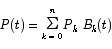
All of the techniques that we look at in this chapter are based on forming weighted averages of a set of control points. Mathematically, this looks like
Because the averages are formed by using so called blending functions, the point that falls out of this process is a function of t. Bezier curves are formed by using four control points in combination with the Bernstein polynomials of order three as blending functions.
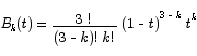
It is possible to extend this method to more control points than four by using higher order Bernstein polynomials, but curves built in this way are difficult to work with.
Some good features of the Bezier curve include
Bad features include
In an effort to address some of the bad points raised here, Bernstein polynomials can be replaced with spline curves. A spline curve is a curve composed of segments that are usually polynomials of relatively low degree. Splines can be sculpted to have desirable shapes and can be made to vanish outside some limited region called the span. This helps with problem 1 above. Because the individual curves usually have fairly low degree splines are not as susceptible to problem 3 above.
Spline curves can be constructed in a variety of ways. One of the most widely used algorithms for constructing spline curves is based on a simple recursive formula:
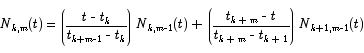
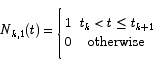
The points tk are called knot points. Roughly speaking, knot points are points at which the various segments that make up the spline are joined together. To completely specify a B-spline curve of order m with L control points we have to specify a knot vector (t0, t1, …, tL + m).
Values in the knot vector can be repeated. If a given t value appears n times in the list we say that that knot has multiplicity of n. The most commonly used knot vector is the so-called standard knot vector in which the first and last knots have multiplicity m and the other knots have unit spacing. In the special case when L is 3 and m is 4, if we choose the standard knot vector (0,0,0,0,1,1,1,1) the B-spline functions reduce to the Bernstein polynomials of degree three and we get the usual Bezier curve.
B-spline curves have all of the desirable characteristics of Bezier curves and additionally avoid problems 1-3 listed above. The one remaining problem is that B-spline curves are not invariant under perspective transformations.
There is however a class of curves based on the B-spline curves which is invariant under perspective transformations. These curves are the Non-uniform rational B-splines, or NURBS for short. These blending functions are computed from the B-spline functions by
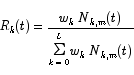
The weight values wk that appear in this formula can be set arbitrarily. The only restriction is that they must all be positive values and they must not all be the same.